In Vitro Fertilization (IVF) - Embryo Quality Grading Based On The Image On Day 3

Introduction

The embryo quality grading is imperative because of the expensiveness to breed an embryo each day. Embryologists usually find patterns from an embryo image in day 3 to decide whether it can develop to day 5 (good) or not (bad). Usually, a decision is based on the subjective thinking and experience of an embryologist. Having a consistent computer-aided scheme to decide will definitely help to improve the performance of the problem.

Problem statement

Two-class image classification problem. Predict whether an embryo can develop until day 5. Assign 'yes' to the embryo image if it can, else 'no'.

Embryo detection/cropping

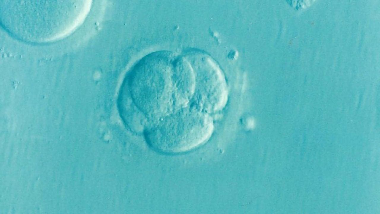
Figure 1: An embryo image (image from [1]).

An embryo image often contains a background. The background is not needed and it contains noises. The stage of detecting the embryo region from the original image will help an algorithm to focus on the right information without being affected by background noises.

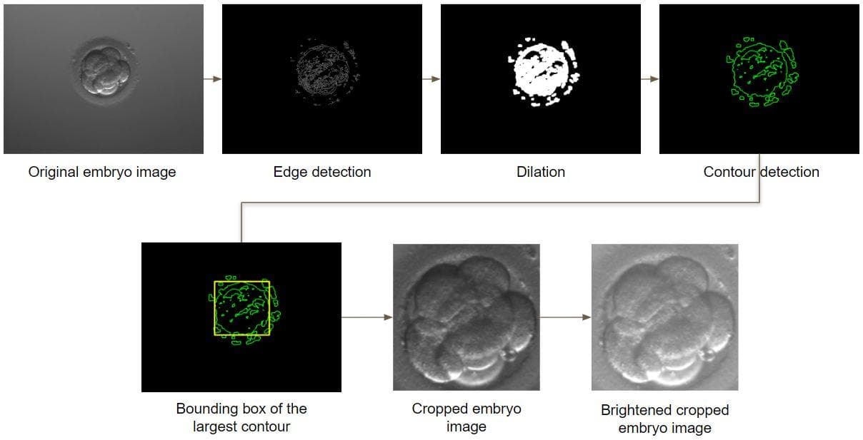
Figure 2: The process of embryo detection, resizing and brightening.

The detection is composed of 5 image processing steps:

• Edge detection: Usually, an embryo image only contains one region that has high density of edges. That is the embryo region. Therefore, when applying a Canny edge detector, we will have an edge image that has mostly white lines (edges) in the embryo region (foreground) and is mostly black in the other regions (background).
• Dilation: Then, the dilation is applied to the edge image so that each collection of near edges will transform into a solid region. Now, the edge image has been transformed. It will have several solid white regions of different shapes and sizes, the other regions is still black.
• Contour detection: Next, use the image processing technique to find contours in the transformed edge image. A contour is certainly found around each solid white region.
• Find the bounding box (coordinates) of the largest contour (the largest contour has a very high chance that it surrounds an embryo): From the collection of contours found above, find the one that has the largest area. Then, use the id of the largest contour to find its bounding box (OpenCV has a function to do this).
• Crop the embryo region: Now, we have already had the bounding box (and its x_min, y_min, x_max, y_max). Use that coordinates to crop the sub-image that fittingly crops the embryo region.

After cropping, each cropped image is resized to have a square shape of size 600x600. Then it is brightened by an ad-hoc algorithm.

Feature extraction

For each embryo image, we need to extract features to represent that image. A representative feature vector usually has a lower number of dimensions of its image, which is supposed to contain only salient information. There are 3 types of features we choose to experiment with. Each type of feature is independently used.

• SIFT [2]: this feature is too popular, if you want to know more about the details, read the paper [2].
• ORB [3]: this feature is an efficient alternative to SIFT and SURF.

• Combination of Contour properties [4]: for each embryo (cropped) image, we use OpenCV to find contours on it. For each detected contour, the list of contour properties below is calculated.

  • area: the area of the contour
  • aspect ratio: the aspect ratio of width to height of the bounding rectangle of the contour
  • equivalent diameter: the equivalent diameter is the diameter of the circle of which area is equal to the contour area
  • extent: the extent is the ratio of the contour area to the area of its bounding rectangle.
  • perimeter: the perimeter (arc length) of the contour
  • solidity: the solidity is the ratio of the contour area to the area of its convex hull
  • mean_color_val: the average color of all pixels in the contour
  • min_gray_val, max_gray_val: the minimum grayscale color and the maximum grayscale color in the contour
  • Hu moments: one purpose of Hu moments is to find how similar two shapes are. There is a good post explaining this at LearnOpenCV.

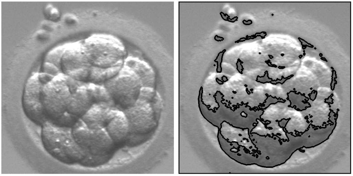
Figure 3: Apply the OpenCV find contours on a cropped embryo image.

When having already extracted features, we will give them to classification algorithms. The algorithm we use to experiment is Bag of Visual Words (BoVW). Note that BoVW needs to be used with K nearest neighbors (KNNs) for classification.

Bag of Visual Words [6, 7, 8]

Supposing that we have two sets of images, one for training and one for testing. The idea of the Bag of Visual Words is:

• First, we need to build a dictionary of words from a pool of extracted features. The extracted features are from images in the training set.
• To build, we need to choose the number of words in the dictionary. Supposing we have F extracted, the number of words K is usually chosen to be less than F (K < F).
• When K is chosen, it is the K (the number of clusterings) in the K-means algorithm. The extracted features are then clustered into different clusters. The centroid of each cluster, which is represented by a D-dimensional vector (D depends on the feature that is used (SIFT is, ORB is, contour is)), is one (visual) word in the created dictionary.
• We use the created dictionary to create a single representative vector for each image (both in the train set and the test set).
• Now, come to the testing stage. To predict a class ('yes' or 'no'), K nearest neighbors is used. From the representative vector of a test image, we find N nearest (e.g. in Euclidean distance) representative vectors of the train set. Then, count whether the number of 'Yes' samples is more than the number of 'No' samples or not. Finally, assign the dominant class to the test image as its predicted label.

You can read more about the details of the Bag of visual words link1 link2 link3.

Deep image classification network

The performance of deep convolutional networks has achieved the state-of-the-art position in recent years in computer vision. It is worth trying different CNN architectures to see how they perform in classifying between good embryos and bad embryos. We try with many network architectures: MobileNetV2, InceptionV3, Resnet50, EfficientNet (B1-B4), DenseNet121, DenseNet169, DenseNet201.

Some experimental results

1) Bag of Visual Words

Below are the best results when using SIFT, ORB, or Contours for Bag of Visual Words. The Kmeans clustering technique is used for creating (visual) words in a dictionary. K nearest neighbors (with K is 3) is used in the testing phase.

Feature extraction	Dimensions of a feature vector	The maximum number of features for each image	Clustering	Number of clusters	Prediction (Test using min distance)	Test accuracy	"No" F1	"Yes" F1
SIFT	128	//	Kmeans	4000	3-NN	0.578	0.613	0.538
ORB	32	500	Kmeans	1500	3-NN	0.549	0.511	0.582
Contour	16	//	Kmeans	50	3-NN	0.578	0.527	0.619

The test accuracy when using SIFT feature is equal to the one when using the Contour feature (~0.578). When looking into the detailed metrics (F1, precision, recall), you can see the differences.

2) Deep image classification network

All the networks are pretrained on ImageNet and have the required input image size of 320x320. For all the training processes, we set the batch size to 9, epochs to 100, and base learning rate to 1e-5. The first two layers are freezed. The reason why most of the layers are unfreezed is that the network weights learned from the ImageNet dataset seem not to be useful for datasets from different domains (IVF is in the medical domain)

Network	Total params	Test accuracy	AUC
MobileNetV2	2,259,265	0.549	0.54
InceptionV3	21,804,833	0.480	0.49
Resnet50	23,589,761	0.569	0.57
EfficientNet-B1	6,576,520	0.529	0.59
EfficientNet-B2	7,769,978	0.490	0.52
EfficientNet-B3	10,785,072	0.559	0.52
EfficientNet-B4	17,675,616	0.451	0.49
DenseNet121	7,038,529	0.519	0.54
DenseNet169	12,644,545	0.588	0.67
DenseNet201	18,323,905	0.559	0.60

The DenseNet169 has the highest test accuracy (~0.588). More information about DenseNet can be found in the paper [9].

3) T-SNE visualization (from the IPython notebook of Scikit-learn link)

From the two experiments 1) and 2) above, the best result belongs to DenseNet169 with a test accuracy is just 0.588. Though there are only 2 classes ('yes' and 'no'), deep networks perform badly in classification. This problem shows that it is very hard to discriminate between good embryos and bad embryos. Let's use T-SNE visualization [10-13] on all the dataset images (both in the train set and the test set) to check if they can be separated into two clusters - 'yes' and 'no'.

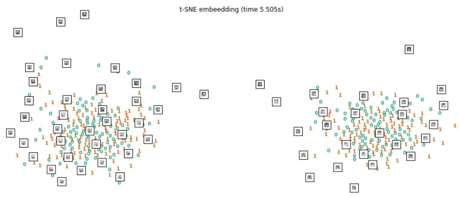
Figure 4: T-SNE visualization.

The blue zeros are 'No' samples, the orange ones are 'Yes' samples. Some embryo images are plotted together. We can see that there are two clusters, but in each cluster, 'yes' and 'no' samples are mixed together. This visualization somewhat shows how challenging the problem is.

Conclusion

In computer vision, embryo quality grading is a new problem. It has received attention in recent years. This problem is related to the life of a human, thus it is very important to have a high-performance and interpretable algorithm that would support embryologists to make their decisions.

References

[1] Doug Donovan, ABNORMAL CELLS IN EMBRYOS MIGHT NOT PREVENT IVF SUCCESS, Johns Hopkins University, 2020.

[2] Lowe, David G. "Distinctive image features from scale-invariant keypoints." International journal of computer vision 60.2 (2004): 91-110.

[3] Rublee, Ethan, et al. "ORB: An efficient alternative to SIFT or SURF." 2011 International conference on computer vision. Ieee, 2011.

[4][contours in opencv](https://opencv24-python-tutorials.readthedocs.io/en/latest/py_tutorials/py_imgproc/py_contours/py_table_of_contents_contours/py_table_of_contents_contours.html)

[5] Cortes, Corinna, and Vladimir Vapnik. "Support vector machine." Machine learning 20.3 (1995): 273-297.

[6] Li Fei-Fei (Stanford), Rob Fergus (NYU), Antonio Torralba (MIT), Recognizing and Learning Object Categories, MIT CSAIL, 2005.

[7] Bethea Davida, Bag of Visual Words in a Nutshell, Towards Data Science, 2018.

[8] Aybüke Yalçıner, Bag of Visual Words (BoVW), Medium, 2019.

[9] Huang, Gao, et al. "Densely connected convolutional networks." Proceedings of the IEEE conference on computer vision and pattern recognition. 2017.

[10] “Visualizing High-Dimensional Data Using t-SNE” van der Maaten, L.J.P.; Hinton, G. Journal of Machine Learning Research (2008)

[11] “t-Distributed Stochastic Neighbor Embedding” van der Maaten, L.J.P.

[12] “Accelerating t-SNE using Tree-Based Algorithms” van der Maaten, L.J.P.; Journal of Machine Learning Research 15(Oct):3221-3245, 2014.

[13] “Automated optimized parameters for T-distributed stochastic neighbor embedding improve visualization and analysis of large datasets” Belkina, A.C., Ciccolella, C.O., Anno, R., Halpert, R., Spidlen, J., Snyder-Cappione, J.E., Nature Communications 10, 5415 (2019).